How to build a CubeSat power budget: solar arrays, batteries, eclipse
Load tables by mode, eclipse fraction, solar-array sizing with EOL degradation, battery depth-of-discharge, and a worked 6U example you can reproduce.

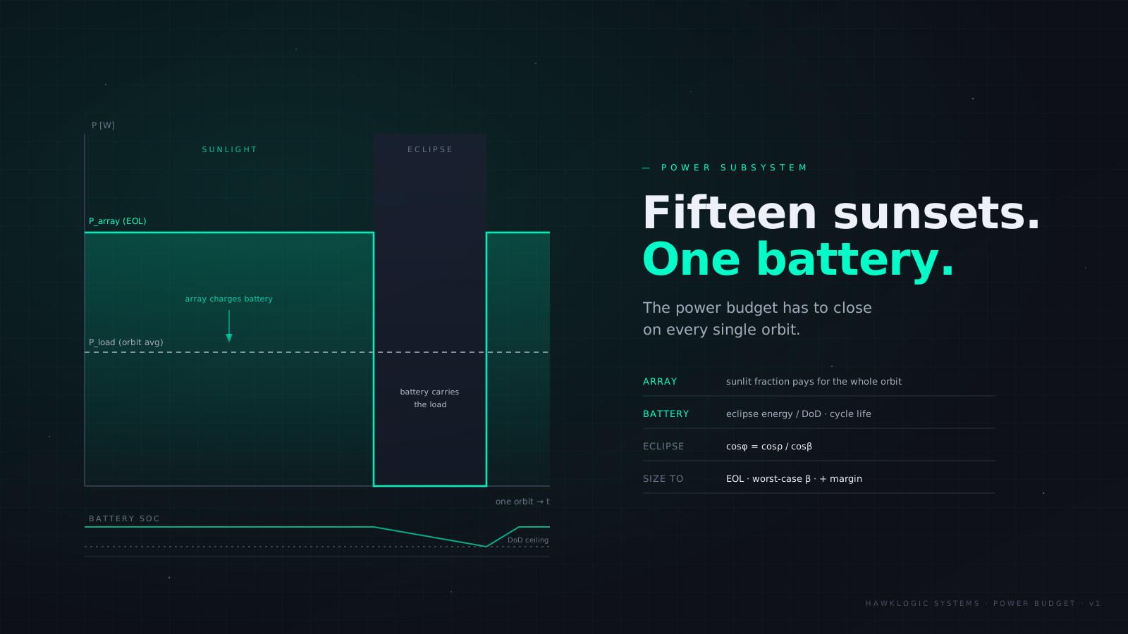
A delta-v budget is spent once. A power budget has to close every orbit, forever: at 500 km that’s about fifteen sunsets a day, each one handing the spacecraft to its battery for half an hour or more. Miss the balance by a few percent and nothing dramatic happens on orbit one; the battery just ends each eclipse slightly deeper than it started, and some weeks later the undervoltage lockout makes the decision for you.
The good news is that first-order power sizing is deterministic arithmetic with well-documented inputs, which means it is checkable in an afternoon. This post walks the standard method (the orbit energy-balance treatment from Space Mission Analysis and Design (SMAD), Ch. 11) and works one CubeSat end to end with numbers you can reproduce in our spacecraft power budget calculator.
Step 1: the load table, by mode
A spacecraft does not draw one number. It cycles between operating modes (safe, nominal, payload-on, downlink), and each mode has its own draw and its own share of the orbit. The honest starting point is a table:
| Mode | Draw | Fraction of orbit | Weighted |
|---|---|---|---|
| Safe | 15 W | 0.15 | 2.3 W |
| Nominal | 29 W | 0.55 | 16.0 W |
| Payload active | 54 W | 0.20 | 10.8 W |
| Downlink | 48 W | 0.10 | 4.8 W |
The orbit-average load is the fraction-weighted mean of the mode draws, here 33.8 W. Two numbers out of this table matter downstream: the orbit average (which sizes the array) and the worst-case mode draw (which sizes the bus regulators and tells you what happens if the spacecraft gets stuck there). Our power budget by mode tool runs exactly this accounting (itemised subsystem draws per mode, fraction weighting, orbit energy balance, and the eclipse depth-of-discharge check), so you can iterate the table without a spreadsheet.
Duty cycle hides in the fractions. A payload that draws 30 W “when on” but is on for 20% of the orbit contributes 6 W to the average. It is very easy to build a budget where every subsystem lead quotes their peak number, everyone adds margin, and the resulting “average” is a stacked worst case that never occurs. Weight by realistic mode fractions, then apply margin once, at the end, where you can see it.
Step 2: orbit period and eclipse fraction
For a circular orbit at altitude h, Kepler’s third law gives the period:
T = 2π · √(a³/μ), a = Re + hWith Re = 6378.137 km and μ = 398600.4418 km³/s², a 500 km orbit has T ≈ 94.6 min, about 15.2 orbits per day.
How much of that orbit is in shadow depends on the beta angle, the angle between the Sun vector and the orbit plane. The spherical-Earth shadow model (SMAD Ch. 5) is compact:
ρ = arcsin(Re / r)                      (angular radius of Earth from the spacecraft)
if |β| ≥ ρ:  no eclipse
else:        cos(φ) = cos(ρ) / cos(β),  eclipse fraction = φ / π
At 500 km, ρ ≈ 68°. With the Sun in the orbit plane (β = 0) the eclipse fraction is 0.378, 35.8 minutes of every 94.6-minute orbit on battery. That β = 0 case is the design-conservative assumption for any low- or mid-inclination orbit, because β sweeps through zero as the orbit precesses and the seasons turn; sizing to a milder beta means the budget stops closing for part of the year.
The exception is a dawn-dusk sun-synchronous orbit (SSO), which rides the terminator and keeps β high year-round, bounded below by 90° minus Earth’s 23.4° axial tilt, i.e. about 66.6° at the winter-solstice worst case. At 500 km that cuts the eclipse fraction to roughly 0.11, which is why power-hungry missions love dawn-dusk SSO. To see how β, and with it your eclipse duration, actually evolves over your mission for a specific orbit and epoch, run the eclipse and beta-angle timeline tool; the worst-case month is the one you size to.
Step 3: sizing the solar array
The array must generate, during the sunlit fraction of the orbit, all the energy the spacecraft consumes over the whole orbit. The full SMAD form separates the two energy paths with their own efficiencies:
P_sa = (Pe·Te/Xe + Pd·Td/Xd) / Tdwhere Pe, Te are the eclipse load and duration, Pd, Td the daylight load and duration, and Xe, Xd the path efficiencies from array to load: through the battery for the eclipse path, direct for the daylight path. SMAD’s reference values: Xe ≈ 0.65, Xd ≈ 0.85 for a direct-energy-transfer (DET) bus; Xe ≈ 0.60, Xd ≈ 0.80 with peak-power tracking (PPT). The eclipse path is worse because every eclipse watt-hour pays the battery’s round-trip toll on the way through.
For preliminary sizing, our calculator uses the condensed energy-balance form, the average load carried across the sunlit period, with path losses and uncertainty folded into a single explicit design margin:
P_array,EOL = (P_avg · T / T_sun) · (1 + margin)Either way, what comes out is a required end-of-life (EOL) power. Getting from there to panel area takes three more factors:
- Cell efficiency. Triple-junction GaAs space cells deliver about 28% at beginning of life (BOL). (Silicon is cheaper and nearer 20%; almost all current smallsat flight hardware is triple-junction.)
- Packing factor. Cells never tile a panel completely: interconnects, hold-downs, and edge keep-outs leave ~85% of the substrate as active cell area.
- Lifetime degradation. Radiation displacement damage, ultraviolet darkening, thermal cycling, and micrometeoroid scuffing erode output over the mission. A combined factor of 0.85, EOL output at 85% of BOL, is representative for a multi-year Low Earth Orbit (LEO) mission; harsher radiation environments do worse.
So the area is:
A = P_array,EOL / (1367 W/m² · 0.28 · 0.85 · 0.85) ≈ P_array,EOL / 277 W/m²with 1367 W/m² the solar constant at 1 AU. Note what that chain of factors does: a “28% efficient” array delivers about 277 usable watts per square metre at end of life, not 383. The gap between those two numbers is where optimistic power budgets go to die.
Step 4: sizing the battery
The battery’s routine job is carrying the load through eclipse. The energy it must deliver per orbit is simply:
E_eclipse = P_avg · T_eclipseBut you cannot cycle a battery from full to empty fifteen times a day and expect it to last. Capacity is set by the depth of discharge (DoD) ceiling, which is a cycle-life decision: a 500 km mission accumulates ~5,500 eclipse cycles per year, so a five-year mission is ~28,000 cycles, and cycle life falls steeply with cycling depth. Typical LEO ceilings by chemistry (SMAD Ch. 11 order-of-magnitude figures):
| Chemistry | Typical LEO DoD ceiling |
|---|---|
| Lithium-ion | ~40% |
| Nickel-hydrogen | ~60% |
| Nickel-cadmium | ~20% |
Li-ion is the modern smallsat norm; a conservative preliminary design sizes to 30% DoD, leaving headroom for the occasional deeper safe-mode excursion. Capacity is then:
C = (E_eclipse / DoD) · (1 + margin)Round-trip efficiency belongs in this step too (a Li-ion charge-discharge cycle returns roughly 90–95% of the energy in), though in the condensed sizing form it rides inside the design margin rather than appearing as its own factor.
For mass, pack-level Li-ion lands around 150 Wh/kg: cell-level state of the art is 180–240 Wh/kg, and harness, battery-management electronics, and mechanical mounts take pack-level to roughly 60–70% of that (NASA Battery Handbook figures).
The worked example: a 6U imaging CubeSat
Take a 6U at 500 km, 51.6° inclination: a rideshare-typical mid-inclination orbit, so β = 0 is the sizing case. Payload draws 20 W at a 30% duty cycle; bus housekeeping is 5 W continuous. Design margin 25%, Li-ion at 30% DoD, and the array factors from Step 3.
| Quantity | Value |
|---|---|
| Orbit period | 94.6 min |
| Eclipse fraction (β = 0) | 0.378 → 35.8 min eclipse, 58.9 min sun |
| Orbit-average load | 20 × 0.3 + 5 = 11 W |
| Array power required (EOL) | (11 × 94.6 / 58.9) × 1.25 = 22.1 W |
| Array power at BOL | 22.1 / 0.85 = 26.0 W |
| Array area | 22.1 / 277 = 0.080 m² |
| Array mass (rigid, 2.8 kg/m²) | 0.22 kg |
| Eclipse energy per orbit | 11 W × (35.8/60) h = 6.56 Wh |
| Battery capacity (30% DoD, +25%) | (6.56 / 0.3) × 1.25 = 27.3 Wh |
| Battery mass (150 Wh/kg) | 0.18 kg |
| Power system mass (incl. 30% overhead on the array) | 0.47 kg |
Two readings of that table are worth pausing on. First, the array must produce twice the average load: 11 W of consumption became a 22 W EOL requirement, because the sunlit 62% of the orbit has to bankroll the whole 100%, at end of life, with margin. Second, 0.080 m² does not fit on one face of a 6U: the long face is 0.06 m², and that’s before the 0.85 packing factor. This spacecraft needs either a modest deployable panel or a payload duty-cycle conversation, and it is much better to have that conversation now than at the structure Critical Design Review.
Every number above comes out of the spacecraft power budget calculator; load the defaults, set the inclination to 51.6°, and you’ll reproduce the table exactly, then stress it: push the altitude down, the duty cycle up, the degradation factor to a harsher 0.75.
Margins and the classic traps
Sizing at BOL instead of EOL. The array that closes the budget on launch day is 15% too small in year five. Every requirement in the budget is an EOL requirement; BOL power is a derived output you quote to the panel vendor, not the thing you size to.
Assuming pointed when you’ll be tumbling. The sizing above assumes an array held at normal incidence to the Sun. A body-mounted CubeSat that tumbles, or that must point its payload nadir while the Sun goes where it will, collects a substantially smaller effective area; the cosine losses are brutal and attitude-dependent. Budget with an effective-area knockdown that matches your actual attitude concept, and remember that safe mode, the mode where you most need power, is usually the mode with the worst pointing.
Sizing at a friendly beta. An eclipse fraction sampled on a mild day of the year is not a design number. Size at worst-case β (zero, for most inclinations), and check the beta timeline for your specific orbit rather than assuming.
Forgetting the balance-of-system. Cells and cells alone are not a power system. Harness, deployment mechanisms, the power conditioning and distribution unit (PCDU), and structural mounts add roughly 30% on top of the array mass for body-mounted designs, more for deployables with hinges and dampers.
Stacked hidden margins. A 25% explicit margin at Preliminary Design Review is healthy and standard. Five subsystem leads each quietly padding their load numbers by 30% before the margin is applied is how a feasible mission gets cancelled on paper.
The full loop (mode table, eclipse geometry, array, battery, margin) is maybe an hour of honest work with the three tools linked above, and it is the difference between a power system that closes by design and one that closes by luck. Run it before the solar-panel purchase order, because orbit-average arithmetic is considerably cheaper to fix than a deployable array.
On this page
Read next
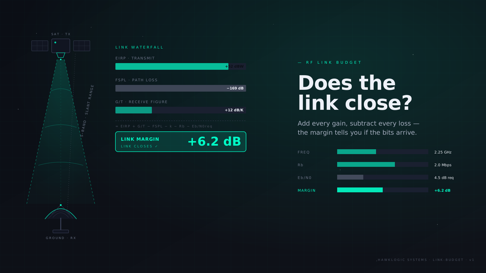
How to build a satellite link budget that actually closes
The full downlink chain (EIRP, back-off loss, FSPL, ITU-R P.618 rain fade, G/T, C/N0, Eb/N0) with a worked 8.2 GHz X-band CubeSat example.
8 min read
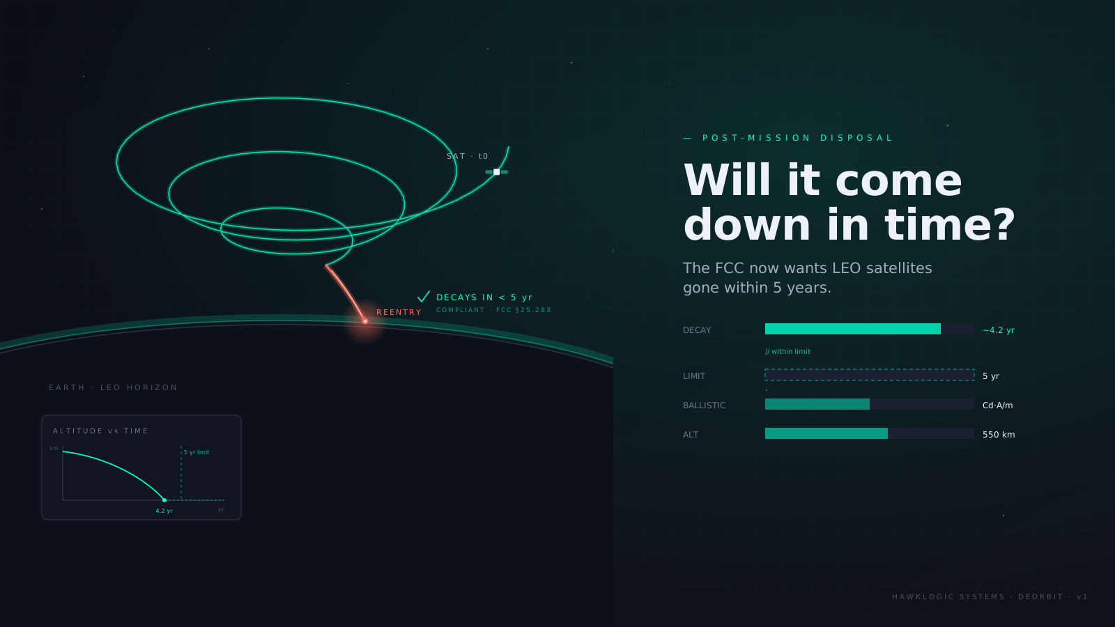
The FCC 5-year rule: will your CubeSat come down in time?
Orbital decay physics, ballistic coefficient, solar-cycle sensitivity, the FCC 5-year post-mission disposal rule, ESA Zero Debris, and remediation options.
8 min read